How many of you wanted to be seated at the corners of your bench or table during school? Well, I preferred it. Why so? It would be easy for me to rush out of the class when the final bell rang. Those days were awesome. Why are we supposed to remember those golden days here? Let’s see.
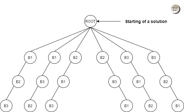
A classic example ahead. Suppose there are three boys (B1, B2, and B3) to be seated on a table. How many possibilities can be extracted? 3! (=6) right! Look at the below diagram for how.
Prerequisite Zone:
State Space Tree: It is a type of tree that represents all the states of the problem without stating if it is the solution or not. It starts from a root as an initial state and continues until the leaf node where it is the terminal state. In our case, Figure 1 is the state space tree.
Backtracking is not an optimization algorithm. It is used when all the possible solutions for a problem are to be extracted and eventually a set of solutions satisfying the constraints laid can be selected. Firstly, we require all the possible solutions. Here is where the Brute Force comes into the picture. Brute Force is a process of finding all the possible solutions to a given problem.
We have got all the possible solutions from the Figure 1 and now we shall put a constraint on the problem. We require B2 to always be seated in the middle. Now, we will find only that set of solutions that satisfy the given constraint.
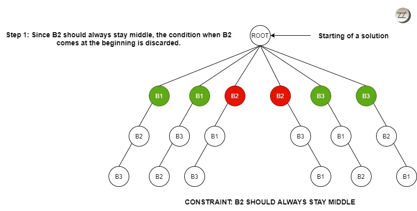
At step 1 (Figure 2.1), the nodes starting with B2 can simply be discarded as the constraint is not satisfied and hence the branch or state can be killed.

At step 2 (Figure 2.2), as B2 is not in the middle, circles marked red in the second state, that particular state can be killed.
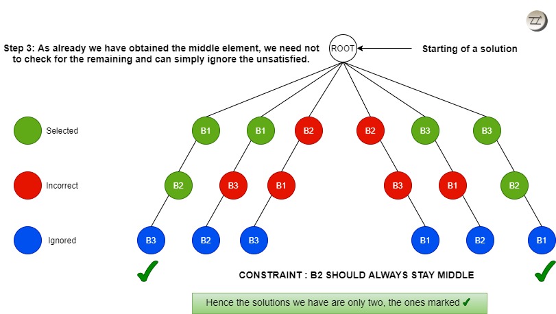
At step 3 (Figure 2.3), we need not check for the leaf node for the solution as the constraint is not satisfied.
Algorithm of Backtracking:
Step 1: if current_position is the target, return success
Step 2: else,
Step 3: if current_position is an endpoint, return failed.
Step 4: else, if current_position is not an endpoint, explore and repeat the above steps.
Summarizing the process of backtracking:
How can backtracking be applied here? In the process of finding solutions to our problem, we encounter many possibilities in our way. But the decision should be taken considering constraints/conditions.
If you see the first parent node, the branch satisfies the condition that B2 should always be in the middle. Hence, that comes out to be one of our solutions. Now we shall look at the second parent node. We found that there is B3 in the next position, middle, which doesn’t satisfy the constraint. So, we simply kill that node or branch and we backtrack ( → )from B3 of the second branch.
This backtracking is followed for all the states and the final solutions are obtained. But the backtracking algorithm has higher time and space complexities. Which is why, many problems are solved using other algorithms such as Dynamic Programming, Greedy Approach, etc. However, there are still some problems that can only be solved using backtracking.
Short information on Tree:
Node: It is a structure in a tree (here) that holds a value.
Root: The node at the top of the tree is root.
Parent: The node which is not the root node and above a node is a parent.
Child: The nodes that are connected to the parent node (s) are child nodes.
Leaf Node: The nodes which do not have any children are leaf nodes.

One thought on “Backtracking”