Reading Time | 7-10 min

In every course about algorithms, the subject of complexity of algorithms is introduced right at the beginning. This implies that the topic plays an important role in understanding algorithms, and I can assure you that it certainly does. Don’t believe me? Read on.

The Need for Speed(complexity)

Every algorithm in computer science requires a computer to run. If in the 1980s, a programmer used a Commodore 64 to run his/her algorithms, then in the future, a programmer may use an even more powerful machine (remember Moore’s Law?). In both cases, the algorithms may not change much or even change at all, but the capability of the hardware changes significantly as time passes. Today, we have enough computing power in our pockets to run highly complex programs with ease, and in a few years, capabilities of such systems will surely increase.

In this case, we need to devise a way to evaluate algorithms independent of the machine being used to run it. This allows us to decisively say that “Algorithm A performs better than algorithm B” and not something like “Algorithm A performs better on a quantum computer than on a classical computer.”.

In basic terms, complexity of an algorithm refers to the amount of resources required to run it, such as time and memory. Since we are talking about time complexity, I have chosen to ignore memory requirements for now. Note that we do not define time in any standard units such as seconds, milliseconds or minutes, since we want the measurement of time to be independent of hardware performance. This is because a faster computer can execute programs faster than a slower computer. An implementation of an algorithm is called a program.

Time Complexity

Time complexity refers to the time taken to run an algorithm, and is proportional to the number of times a basic operation is executed. The basic operation is that which consumes longest amount of time while executing. We also assume that the time taken to complete each basic operation is constant. However, the time taken to run an algorithm varies depending on the input size. Let me give an example.

Assume that a single dimensional array A is given. The array is a zero indexed array, i.e. the first element is at position 0, second element at position 1 and so on.
A = {3, 1, 4, 5}
Linear search algorithm is used to search for an element from a vector/tuple/array. It works by checking every element of the array until the element is found or the end of the array is reached. After a successful search, the algorithm returns the position of the element within the array. We assume that the search begins from the lowest index, i.e. 0. Let us try to find 2 different elements using this algorithm.

Case 1: Finding element 3

We will use the algorithm to search for the number 3. It will find the element at the zeroth position of the array, hence stopping after performing just one comparison.

This means that the shortest execution time for linear search is observed when the element being searched is in the zeroth position, thus implying that the time taken to search is constant (in real life, this constant will be some amount of time like 100ms, but since we are talking about complexity, we only mention it as a constant).

Case 2: Finding element 6

On the other hand, if we use the algorithm to search for 6, then the algorithm will search through A without finding an element which is equal to 6. In this case, the algorithm performs 4 comparisons, since there are 4 elements.

Generalizing the second case, assume that the array has n elements. The longest execution time(i.e. the worst case complexity) would be the case when the element being searched is not in the array. In this case, n comparisons will be made, and so the time complexity is assumed to be linear (a function of n).

This means that if we replaced the A with A={100, 99, 98, 97, ..., 1} and try to apply the same algorithm to find element 0, we will notice an increase in execution time (in the worst case) proportional to the increase in size of the array. No change will be observed in the best case complexity.

The first case is said to be the best case time complexity since it is the shortest time in which an element can be found.

Case 3: Finding any element

In case of linear search, the average case complexity is the average time required to find an element in an array of size n.

Among the three cases, the worst case complexity is often assigned a higher priority, along with the average case complexity. Using the three cases and the example, I hope I have convinced you that running time of an algorithm varies. In general, if an input of size n is given, then the running time varies as a function of the number of times the basic operation is executed. If we represent running time by T(n), the number of executions of a basic operation as C(n), and the time taken for execution of a single basic operation as cop, then:

T(n) ≈ cop * C(n)

T(n) is almost equal to the R.H.S. since in some cases, other operations also take some time to execute. One such operation is the assignment of variables.

Running Time and Basic Operations

An algorithm comprises of multiple steps, each of which may take different amounts of time for execution. A basic operation is usually that operation which takes the longest to execute. Take a look at the following algorithm to print a half triangle.

Algorithm HALF_TRIANGLE:
Given an integer m, let t denote the integer corresponding to the line being printed (t ≤ m) and n be the number of * characters printed on a single line (n ≤ t). Display * characters on each line such that the number of * characters on each line is equal to the line being printed, for example line number 4 should have four * characters.

• S1:[Check m] If m ≤ 0, terminate
• S2:[Initialize t] t ← 1
• S3:[Move from line] While t ≤ m do:
             n ← 1
             Go to S4
             t ← t + 1
          done
• S4:[Display *] While n ≤ t do:
          display ‘*’
          n ← n + 1
        done
        Go to S5
• S5:[Go to next line] Move cursor to next line.
• S6:[End] Terminate

You can see that the two statements in the while loop (S4) are executed the largest number of times. If m = 5, then each statement executes a total of
1 + 2 + 3 + 4 + 5 = 15 times in the inner loop.

Generalizing,

If m = n where n is any positive integer, then the total number of times the two statements will be executed inside S4’s while loop is given by:
1 + 2 + 3 + 4 + … + n = (1/2)* n * (n+1)
=(n²/2) + (n/2)

Now, we know that for very large values of n, (n²/2) > n/2.
We can ignore the term (n/2) in the R.H.S. since the maximum contribution to execution time is from the (n²/2) term.

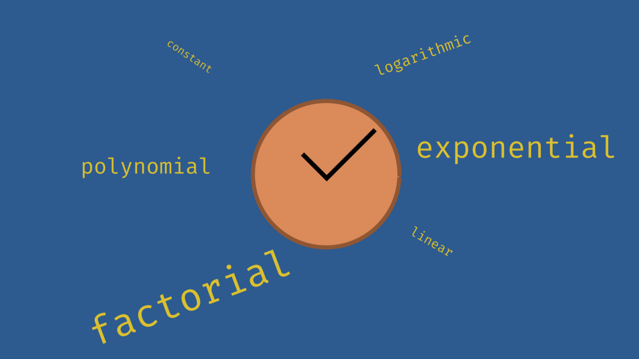
Orders of Growth

Taking this simplification further, to represent the time complexity as a function of n, we introduce the concept of orders of growth. An order of growth is a function which describes the increase in execution time as the input size increases.
Let T(n) be a function representing the execution time of an algorithm. In the algorithm to print a half triangle, T(n) increases as a factor of n² as the number of lines to be printed increases. This is because the statements within the innermost loop are executed more. If the outermost loop in the algorithm is executed n times, then for each iteration of the outermost loop, the innermost loop is executed n times too. This makes the inner statements execute n² times in total. So we can say that the execution time of the algorithm to display a half triangle grows in the order of n².

Enfin

I hope this post was helpful to understand the concept of time complexity. In another post, I’ll be explaining asymptotic notations, which are closely related to the best, worst and average case time complexities. Stay tuned and connected.